Simulation Modeling--Part 3
Let's take a look at a simple order- fulfillment process for a typical company and discover why process simulation is necessary.
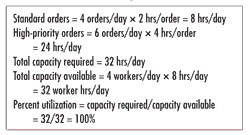
 On average, 10 orders are received every day. On average, 10 orders are received every day.
 Forty percent of the orders are standard and 60 percent are high priority. Forty percent of the orders are standard and 60 percent are high priority.
 On average, standard orders take two hours to process and high-priority orders take four hours. On average, standard orders take two hours to process and high-priority orders take four hours.
 Four workers process orders in eight-hour shifts. Four workers process orders in eight-hour shifts.
Based on the simple calculations shown below, we can conclude that customers will always receive their orders on time and that the order-fulfillment process is optimized with its resources at 100-percent utilization.

Now let's look at a typical day, where the order arrival rate is random. The first two orders arrive at 9 a.m. The third order arrives at 10 a.m. The first three orders are standard orders. At 11 a.m., the first two orders are shipped. Also at 11 a.m., a high-priority order is received. At noon, the third standard order is shipped while two new orders arrive; one is standard, the other high priority. At 12:30 p.m., another high-priority order arrives. At 1 p.m., three more high-priority orders are received. By 4:30 p.m., the workers have shipped seven orders. Three workers stay on and complete the remaining three orders by 8 p.m.
At 1 p.m., the total number of orders in process peaks at seven. The last three orders spend 1.5 hours, two hours, and three hours in queue, respectively. The calculations below summarize the performance measures of the manual simulation.

Although the process appears to be designed perfectly, the random arrival rate of customer orders causes queuing and subsequent delays in processing time. Now, let's take a look at three other possible scenarios.
 What if the business receives anywhere from eight to 12 orders a day (and the most likely daily demand remains at 10 orders)? What if the business receives anywhere from eight to 12 orders a day (and the most likely daily demand remains at 10 orders)?
 What if the time to process high-priority orders is anywhere from three hours to five hours (and the most likely processing time remains at four hours)? What if the time to process high-priority orders is anywhere from three hours to five hours (and the most likely processing time remains at four hours)?
 What if the order mix is random? What if the order mix is random?
How long will it take to fulfill an order (i.e., the cycle time) given the new demand, process times and product mix? The answer is difficult to compute without simulation modeling, because more variability in the process means more variability in performance. Possible results for the cycle times for three scenarios might look like the outcomes in the following table, which shows the average values as well as the values for the mathematical variance (s) in terms of the 2-s variance.

Mathematical variance is important in analyzing the performance of a process. Assuming that observations are from a normally distributed population, the 2-s band contains 95.45 percent of the observations, and the 3-s band contains 99.73 percent.
Customers are lost because of exceptionally bad performance, not average performance. In the scenarios described above, the maximum cycle-time values are outside the 2-s band, representing exceptionally bad performances. The likelihood of a high-priority order taking 7.13 hours is less than 5 percent. Even though this seems like a small percentage, that's all it might take for a major customer to consider doing business with a competitor.
Of course, when a rare event like an exceptionally bad performance occurs, management begins asking questions, including, "How much will be spent in marketing to lure back lost customers?"
If it typically costs x to keep a present customer, it costs 10x to get a new customer and 100x to win back a lost customer. Your priority should always be on keeping your present customers because you can't afford to try to win them back.
This exercise presents a simplistic view of an order-fulfillment process, but it demonstrates the effect of process dynamics on cycle time, service level and process costs. As randomness of behavior and interdependencies of resources increase in a process, it becomes impossible to predict performance without process simulation.
Note: For more information, read Simulation Modeling Methods, a book and CD by H. James Harrington and Kerim Tumay (McGraw-Hill, 2000).
H. James Harrington is CEO of the Harrington Institute Inc. and chairman of the board of Harrington Group. Visit his Web site at www.harrington-institute.com.
|