Black Belt Bound
Michael J. Cleary, Ph.D.
mcleary@qualitydigest.com
When he joined Greer Grate
& Gate as quality manager, Hartford Simsack told his
plant manager and brother-in-law, Rock DeBote, that he'd
really prefer the job of production manager. However, because
DeBote had given Simsack a job after he was released from
prison, he didn't complain too vociferously. Instead, he
set about trying to convince his boss of his eminent suitability
for the production job.
Simsack's son, who is enrolled in martial arts classes,
has quickly moved to Black Belt status, and this gives Simsack
an idea. "If I could only be a Black Belt, that would
impress DeBote," he thinks. "And it can't be too
hard, if an 11-year-old kid can do it."
Simsack selects a project that he believes will save the
company almost $1.5 million. He tracks the percentage of
defects on extruded wrought-iron railings--the plant's primary
output--and, by using a p-chart, anticipates clear analytical
support for his assertion about savings.
The railings are produced in lots varying from 50 to 200
capacity. Simsack dismisses the relevance of variable sample
sizes for p-charts. "I'll just use the average sample
size," he tells himself. But when he looks at the data
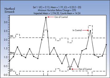
on his printout, the changing control limits confuse him.
Greer Grate & Gate p-Chart

While Simsack examines the printout, Rock DeBote stops
by and finds the charts unclear. "Why do the control
limits go up and down like this?" he asks. "Well,"
Simsack blurts out with mock confidence, "obviously,
this can be attributed to application of the binomial theorem."
What in the world does the binomial theorem--a term he heard
in one of his statistics classes--have to do with the issue
of control limits?
The answer is nothing. Simsack is once again bluffing.
However, p-charts are in fact based on the binomial theorem,
which has everything to do with the appearance of the charted
control limits:


If all samples were the same size--for example 100, the
n-bar would equal 100. In Simsack's case, the sizes vary
from 50 to 200. The printout shows that the average sample
size is 1,194.32. The most common rule is that no adjustment
will be made to the control limits if the sample sizes vary
by no more than 25 percent. On Simsack's charts, it's clear
that sample size varies by more than 25 percent, and an
adjustment to the limits must be made.
Mathematically, the adjustment involves substituting the
actual n of the sample with n-bar. This is done only when
n varies by 25 percent or more from n-bar. Next month's
column will offer an intuitive explanation of this methodology.
Michael J. Cleary, Ph.D., is a professor emeritus at Wright
State University and founder of PQ Systems Inc. He has published
articles on quality management and statistical process control
in a variety of academic and professional journals. His
Web site is www.pqsystems.com.
Letters to the editor regarding this column can be e-mailed
to letters@qualitydigest.com.
|