![](/sites/default/files/editorial_images/Wheel1000_2.jpg)
Photo by bruce mars on Unsplash
The four common capability and performance indexes collectively contain all of the summary information about process predictability, process conformity, and process aim that can be expressed numerically. As a result, any additional capability measures that your software may provide can only repackage what is already known. This article will contrast and compare the so-called third-generation capability ratios with the traditional capability indexes.
ADVERTISEMENT |
The capability indexes
The capability ratio, Cp, is an index that addresses the question, “Is there enough elbow room for my process within the specifications?” It answers this question by comparing the total space available within the specifications with the space required by the process:
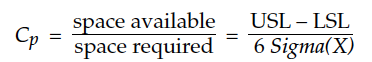
And this ratio is an index number because a value of 1.00 is the borderline between positive and negative answers to the question posed. Here, values greater than 1.00 indicate that the process has adequate elbow room.
The centered capability ratio, Cpk, is an index that addresses the question, “Is my process safely within the specification limits?” It answers this question by comparing the effective space available with the space required by the process.
This index computes the elbow room as if the process was centered within specifications having a tolerance equal to twice the distance between the average and the nearer specification. This ratio is an index number because values greater than 1.00 indicate that, even with the current average, the process still is safely within the specifications.
As the process average approaches the midpoint of the specifications, the centered capability ratio will approach the capability ratio. So, collectively these two capability indexes describe how well-centered the process is relative to the specifications.
These two capability ratios are concerned with the process potential. They describe the actual capability of a process that is being operated predictably, and they describe the hypothetical capability of a process that has been operated unpredictably in the past. However, since performance can fall short of potential, we will also need performance indexes.
The performance indexes
The performance indexes use a different measure of dispersion than the capability ratios use. While the capability indexes use the within-subgroup dispersion, Sigma(X), to describe the process potential, the performance indexes use the global standard deviation statistic, s, to summarize the past performance. Of course, when a process is performing up to its full potential, these two measures of dispersion will converge and the performance indexes will approach the capability indexes from below.
The performance ratio, Pp, is an index that addresses the question, “Was the space used by the process in the past less than the specified tolerance?” It answers this question by comparing the total space available with the space used in the past:
This ratio is an index number because values greater than 1.00 indicate that the specified tolerance has been wider than the historical product stream.
The centered performance ratio, Ppk, is an index that addresses the question, “Has the product stream been safely within the specification limits in the past?” It answers this question by comparing the effective space available with the space used by the process in the past:
This ratio is an index number because values greater than 1.00 indicate that the product stream has been safely within the specifications in the past.
The closer the historical process average has been to the midpoint of the specifications, the closer the centered performance ratio will be to the performance ratio. Moreover, we can judge how predictable the process has been by how closely the performance indexes match the capability indexes.
Using capability indexes
There are known relationships between the traditional capability and performances indexes. These relationships come from the formulas and are summarized in Figure 1.
Figure 1: Relationships between capability and performance indexes
The top row summarizes the process potential—what will happen when the process is operated predictably.
The bottom row summarizes the process performance. When a process is operated unpredictably, its performance will fall short of its potential, and the performance ratios will be smaller than the capability ratios.
The left-hand side summarizes both potential and performance when the process is centered within the specifications, while the right-hand side summarizes what happens when the process is off-center.
Combining all of the above, we see that the gap between the centered performance ratio and the capability ratio will characterize the difference between the past process performance and the process potential. This gap will define the opportunities that exist for improving any process.
The following examples will show how these four capability and performance indexes summarize key aspects of the process, and how the process behavior chart and histogram provide details to finish telling the story.
The socket thickness
Ninety-six data collected over a one-week period had an average of 4.66, a Sigma(X) value of 1.80, and an s statistic of 1.868. The values are the thicknesses in excess of the minimum spec, so negative numbers are possible here. The specs for the coded data were –0.5 to 15.5. Our four indexes are:
The capability ratio tells us that the specified tolerance is 148% of the space required by this process.
The centered capability ratio of 0.95 tells us that the process is not centered in the specs.
The performance ratio 0f 1.43 is essentially the same as the capability ratio; hence, this process has been operated in a reasonably predictable manner.
The centered performance ratio of 0.92 suggests that there is a possibility of 0.4% nonconforming product.
Thus, these four capability and performance indexes capture the highlights for these data. For the rest of the story, we look at the graphs. The histogram shows this process to have a short lower tail. The reason for this short lower tail is a characteristic of this process; that is well understood. So the supervisor knew that the process had not yet reached the point of producing nonconforming product. The off-center operation was the result of six months of tool wear, and shortly after these data were collected the die was retooled to bring the average back up to the target value of 7.5.
Figure 2: Socket thickness average and range chart plus histogram
The density data
During the course of one week, 33 measurements of the density of yarn going into a single strand of material (called a “roving”) were obtained. The average was 523.9, the Sigma(X) value was 4.34, and the global standard deviation statistic, s, was 9.71. The specs were 410 to 550. Our four indexes are:
The capability ratio of 5.38 tells us that the specifications are more than five times wider than the space required by this process. The difference between the capability and performance ratios tells us that this process has been operated unpredictably. And the centered performance ratio of 0.89 tells us that this process has recently been operated close to a specification limit.
When we look at the graphs, we confirm everything suggested by the capability and performance indexes and add the detail that this process is subject to sudden and dramatic changes in level.
Figure 3: Density data 1 chart and histogram
The resistivity data
Sixty-four measurements of the resistivity of an insulating material had an average of 4,418, a Sigma(X) value of 178, and a global standard deviation statistic, s, of 184. The specs were 4,000 to 4,800.
Our four indexes are:
When all four capability and performance indexes converge to similar values as these do, we know that the process is reasonably predictable and centered within the specifications. With ratios in the range of 0.69 to 0.75, we also know that this process may produce about 3% nonconforming.
Figure 4: Resistivity average chart and histogram
As these three examples show, while the process behavior chart and histogram tell the whole story, the four common capability and performance indexes complement the graphs with numerical summaries of the overall process performance and potential.
Off-center targets
But what if the target value is not at the midpoint of the specifications?
Rivets on the skin of an airplane are intended to be flush. Thus, their target value for flushness is 0 mils. The specs for flushness are –2 mils to +1 mil.
When the target value is not at the midpoint of bilateral specifications, you are essentially operating with two one-sided specs where each specification is concerned with a different problem. Here the +1 mil spec is concerned with drag in flight, while the –2 mil spec is concerned with structural strength as well as drag.
In situations like this, I prefer to deal with each specification separately by computing a centered capability ratio for each specification. This allows each of the two separate problems to be addressed, rather than lumping them together in a single computation that can only create confusion.
Third-generation capabilities
Third-generation capabilities claim to characterize how well a process is doing in regard to operating on-target. They seek to do this by tweaking the formulas for capability. They replace the Sigma(X) value with a composite function that includes the square of the distance between the average and the target. These “third generation” capability ratios have been around at least since the ’90s, when they were known as “modified” capability ratios.
The modified capability ratio is Cpm:
where MSD(T) is a modified version of the mean square deviation about the target value, T:
Likewise, the modified centered capability ratio is Cpmk:
As may be seen in the last term above, the ratio of Cpmk to Cpm will be identical to the ratio of Cpk to Cp, so these modified capability ratios tell us nothing new about how well-centered the process is relative to the specifications. They simply deflate the traditional ratios by dividing by a larger quantity.
Of course, by changing the denominator, these third-generation capability ratios change the comparison being made. The traditional capability ratios compare the tolerance or the effective space available with the space required by the process. These modified capability ratios compare the tolerance or the effective space available with a value that is six times the radius of gyration of the histogram about the target value.
This denominator for the modified capability ratios is intended to define the space needed to swing the whole process around about the target value. But since we don’t intend to rotate our process about the target value, the denominator of these modified capability ratios tends to overstate the damage due to being off-target.
Socket-thickness data
The socket-thickness data came from a capable and predictable process that was being operated slightly off-target. Figure 5 compares the specified tolerance of 16 units with four intervals. First is the interval defined by the denominator of the capability ratio (10.8 units). Next is the interval defined by the denominator of the performance ratio (11.2 units). Third is the interval defined by rotating the performance interval (and the histogram) about the target value (16.88 units). And finally we have the interval defined by the denominator of the modified capability ratio (20.17 units).
Figure 5: The socket-thickness histogram rotated about target
This process had been operated predictably and capably for the past six months. The average was 28 microns below the target value due to six months of tool wear. The average was not going to be swinging around the target value in the manner implied by the modified capability ratios.
Knowing that these data have a Cpm ratio of 0.79 and a Cpmk ratio of 0.51 adds nothing to our story. These ratios make things sound much worse than they are by comparing the space available with an imaginary quantity that has no basis in practice.
Density data
The density data came from an unpredictable process with wide specifications that was being operated way off-target. Figure 6 compares the specified tolerance of 140 units with four intervals. First is the interval defined by the denominator of the capability ratio (26.0 units). Next is the interval defined by the denominator of the performance ratio (58.3 units). Third is the interval defined by rotating the performance interval about the target value (146 units).
And finally we have the interval defined by the denominator of the modified capability ratio (266 units).
Figure 6: The density histogram rotated about target
Knowing that the density data have a Cpm ratio of 0.53 and a Cpmk ratio of 0.20 adds nothing to our story. These ratios compare the space available with a quantity that is unrelated to anything we do in practice.
“But doesn’t the modified capability ratio tell us when we are on-target?” Not exactly. The modified capability ratio will exceed 1.00 when we are in the neighborhood of the target, as may be seen in Figure 7. But it doesn’t mean that the process is centered on the target value.
Figure 7: Region where the modified capability ratio exceeds 1
In order for the process to be on-target, the modified capability ratio will have to converge to the traditional capability ratio. Thus, the modified capability ratios are not index numbers where values greater than 1.00 indicate on-target operation.
Resistivity data
The resistivity data came from a process that was operated predictably and on-target, but which wasn’t completely capable. Here the Cpm ratio of 0.74 and a Cpmk ratio of 0.71 converge to the traditional capability indexes because the bias term essentially disappears from their denominator as the process gets near the target. So, once again, these third-generation capabilities add nothing to our story.
Figure 8: The resistivity histogram is on-target
Here we have an on-target process with modified capability ratios that are less than 1.00. When you want to know if your process has been on-target, it’s much easier to use the histogram than to get lost trying to interpret complex numerical summaries such as the modified capability ratios.
Summary
The four capability and performance indexes in Figure 1 contain all of the information regarding the relationship between specifications, process potential, and process performance that can be found in numerical summaries. Collectively, they are a set of sufficient statistics. Once you know these four indexes, additional computations can only repackage what you already know. So if your software offers other capability measures, you should know that they provide nothing new. Modified capability ratios simply add complexity without clarity.
So, rather than telling others the value of one or another of the capability ratios, interpret the four traditional indexes together and tell others whether the process is being operated predictably or unpredictably. Tell them whether the process has been centered in the specifications. Tell them what the fraction nonconforming has been. These are the things they need to know. As these interpretations generate questions, you can then turn to the process behavior chart and histogram to fill in the details.
The operational definition of an unpredictable process is a process behavior chart. It alone, of all the various analysis techniques, preserves the evidence contained in the time-order sequence of the data. This is why numerical summaries can never tell the whole story. The traditional capability and performance indexes can tell part of the story and can complement the process behavior chart and histogram, but they can’t replace the charts. To fully tell the story, you will always need to return to the process behavior chart and the histogram.
Caveat
As if the complexity weren’t already great enough, some software packages may compute the denominator for the third-generation capability ratios using the global standard deviation statistic, s, rather than the within-subgroup variation, Sigma(X). While this change is algebraically correct for computing the mean square deviation about the target, it changes the interpretation of the result. Here, you end up with third-generation performance ratios that add nothing to what is already known.
Comments
Stability Index
The other capability statistic that I see being used is the Stability Index, which is gained by dividing the Cpk by the Ppk or alternatively, Cp divided by Pp. Again, this seems like repackaging already gathered information from the four main indices, though, I think.
Add new comment